Some details about the K-nearest neighbors( KNN )
KNN was proposed by Hart and Cover, whose original purpose is accomplishing the text classsification work. [1] The basic principle behind this algorithm is that, for a given unclassified sample X, we can calculate the likelihood between X and the training set then find K samples that are most similar with the sample X, therefore we are now able to estimate the value of X based on the most common labels among the chosen K samples.
This algorithm is constructed on the limited neighbor samples rather than the region the sample belongs to. Due to this KNN is much more valuable for sample sets that exists many crossover or overlaps within which.
the algorithm realization process
There exists several kinds of implementation method, the key difference between them lies on the choice of “distance” between neighbor samples. I’ll explain that in the following steps. Now we are going to just focus on the traditonal way.
-
At first we need to build our training set. Name it as \(\omega\),
\(\omega = \left \{ \left ( x_i,c_i \right ) \right |i=1,2\cdots n\}\) ,where x is a vector in dimension l, \(x_i^h\) shows the value h in sample i, \(c_i\) means the category that sample i belongs to. -
Then we usually choose an initial value of K and make some adjustments in accordance with our training result. I need to mention that we are used to choosing K as an odd value such as 3, 5, 7. Here for simplicity I’ll take 3.
-
Name the test set as \(\varphi\), \(\varphi = \left \{ y_j|j=1,2,\cdots ,m \right \}\) ,where \(y_j\) is the value h in test sample j. Then it comes to the vital step: calculating the “distance” between neighbours. For example, the distance between training sample i and test sample j is
- Find the nearest K samples in our training set to test sample \(y_i\), name them as \(x_1\), \(x_2\), \(\cdots\),\(x_k\). Now we need to classify them. Construct a discrete function f.
-
If \(m=n\) then we have \(\delta(a,b)=1\), otherwise \(\delta(a,b)=0\). \(\hat{f(y_i)}\) is the category of \(y_i\).
-
Change the value of K, redo the process 3,4,5. Specify K with the best classfication result.
Simple Relization of KNN
ALL attached codes are writeen on Python3.6
You may find that the code does not work on your computer, one possible reason is that you do not install packages involved in my code.
import math
## 三个数字从左至右分别为汽车在内饰、舒适度以及操控性上的得分表现,在此只用于展示,并非真实情况。
car_data= {"CLS 300": [25, 13, 8, "Mercedes-Benz"],
 "C 200L": [31, 10, 10, "Mercedes-Benz"],
 "S600": [38, 17, 4, "Mercedes-Benz"],
 "S63L 4MATIC+": [35, 12, 9, "Mercedes-Benz"],
 "530i": [10, 9, 36, "BMW"],
 "640i": [11, 12, 33, "BMW"],
 "325i": [6, 4, 27, "BMW"],
 "425i": [9, 7, 35, "BMW"],
 "GS450h": [9, 33, 6, "LEXUS"],
 "LX570": [11, 37, 10, "LEXUS"],
 "LS500": [10, 40, 3, "LEXUS"],
 "LC500h": [4, 29, 17, "LEXUS"]}
x = [32,11,17]
KNN = []
for key,v in car_data.items():
  d = math.sqrt((x[0] - v[0]) **2 + (x[1] - v[1]) **2 + (x[2] - v[2]) **2)
  KNN.append([key,round(d,2)])
print(KNN)
KNN.sort(key=lambda dis : dis[1])
print(KNN)
KNN = KNN[:5]
print(KNN)
labels = {"Mercedes-Benz":0,"BMW":0,"LEXUS":0}
for s in KNN: label = car_data[s[0]]
labels[label[3]] += 1
labels = sorted(labels.items(),key = lambda l: l[1],reverse = True)
print(labels,labels[0][0],sep = '\n')
The result has been shown below:
[['CLS 300', 11.58], ['C 200L', 7.14], ['S600', 15.52], ['S63L 4MATIC+', 8.6], ['530i', 29.14], ['640i', 26.42], ['325i', 28.72], ['425i', 29.48], ['GS450h', 33.67], ['LX570', 34.15], ['LS500', 39.0], ['LC500h', 33.29]]
[['C 200L', 7.14], ['S63L 4MATIC+', 8.6], ['CLS 300', 11.58], ['S600', 15.52], ['640i', 26.42], ['325i', 28.72], ['530i', 29.14], ['425i', 29.48], ['LC500h', 33.29], ['GS450h', 33.67], ['LX570', 34.15], ['LS500', 39.0]]
[['C 200L', 7.14], ['S63L 4MATIC+', 8.6], ['CLS 300', 11.58], ['S600', 15.52], ['640i', 26.42]]
[('BMW', 1), ('Mercedes-Benz', 0), ('LEXUS', 0)]
BMW
That is, BMW.
The aplication of KNN with IRIS dataset
Recently I get intouched with a new powerful dataset called scikit-learn, which contains varities of data can be put into the pratice. Here I’ll use one component called IRIS to do some KNN applications.
from sklearn import datasets
iris=datasets.load_iris()
from pylab import *
The code above is used to import data.
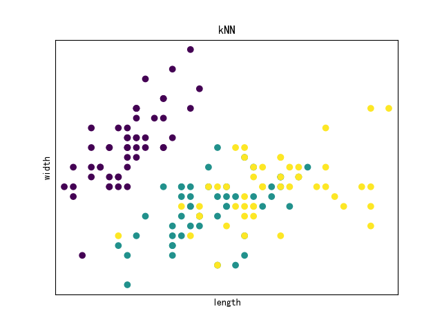
Now I will visualize the Iris data with scatter plot.
import matplotlib.pyplot as plt
x=iris.data[:,0]
y=iris.data[:,1]
species=iris.target
plt.figure()
plt.title('kNN')
plt.scatter(x,y,c=species)
plt.xlabel('length')
plt.ylabel('width')
plt.xticks(())
plt.yticks(())
plt.show()
Here is the result:
Fitness check:
from sklearn import datasets
import matplotlib.pyplot as plt
import numpy as np
from sklearn.neighbors import KNeighborsClassifier
np.random.seed(0)
iris=datasets.load_iris()
x=iris.data
y=iris.target
i=np.random.permutation(len(iris.data))#打乱顺序
##135 training sets and 15 test sets
x_train=x[i[:-15]]
y_train=y[i[:-15]]
x_text=x[i[-15:]]
y_text=y[i[-15:]]

knn=KNeighborsClassifier()
knn.fit(x_train,y_train)
print(knn.predict(x_text),y_text)

##result= [1 2 2 0 1 1 2 1 0 0 0 2 1 2 0] [1 2 2 0 1 1 1 1 0 0 0 2 1 2 0]
The fitness outcome is not that satisfying, we need to draw the boundary of data points through KNN method to have a deeper thought.
from sklearn import datasets
import matplotlib.pyplot as plt
from matplotlib.colors import ListedColormap
import numpy as np
from sklearn.neighbors import KNeighborsClassifier
from pylab import *

## identify the dimension of our data.
iris=datasets.load_iris()
x=iris.data[:,:2]
y=iris.target

x_min,x_max=x[:,0].min()-0.1,x[:,0].max()+0.1
y_min,y_max=x[:,1].min()-0.1,x[:,1].max()+0.1

#this is used for back colour settings.
cmap_light=ListedColormap(['#7F7FFF','#FFAA00','#9999FF'])
h=0.01
xx,yy=np.meshgrid(np.arange(x_min,x_max,h),np.arange(y_min,y_max,h))

# do the pic job
knn=KNeighborsClassifier()
knn.fit(x,y)
z=knn.predict(np.c_[xx.ravel(),yy.ravel()])
z=z.reshape(xx.shape)
plt.figure()
plt.pcolormesh(xx,yy,z,cmap=cmap_light)

plt.title('KNN')
plt.scatter(x[:,0],x[:,1],c=y)
plt.xlim(xx.min(),xx.max())
plt.ylim(yy.min(),yy.max())
plt.xlabel('length')
plt.ylabel('width')
plt.show()
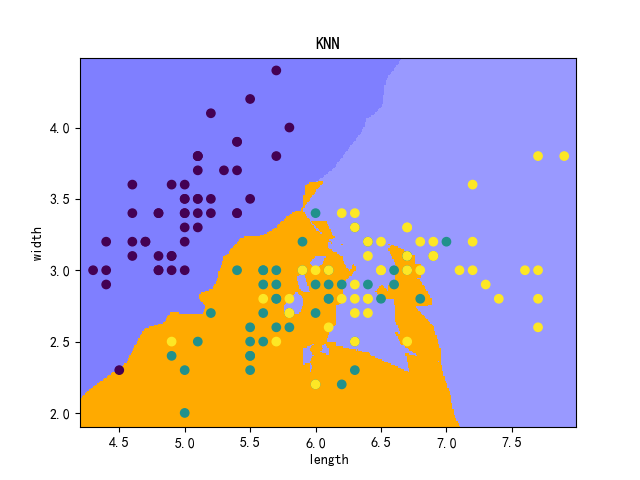
From the given chart we could capture the information that there exists many overlaps in the lower right corner. As you can see, KNN has its limitations, maybe that deserves my deeper research, thank you.