the Variance Inflation Factor( VIF ).
What’s the mutlicollinearity?
The multicollinearity arises when there is any departure from orthogonality in the set of regressors and get worse as the correlation among explanatory variables increase.
To the best of my knowledge, there are two effects, I mean, harms that multicollinearity leads to. On the one hand, the strong correlation among explanatory variables induces numerical instability in the estimates of both regression and statistical tests. The \(\widehat{\beta}\) is very likely to be overestimated and the confidence interval is too loose to be of any practical use. On the other hand, it’s not surprising to observe an increased R-square despite the reduced number of individual significant coefficients, also the t-statistic just fail to present the real pic.
How to assess it?
A simple way to detect collinearity is to look at the correlation matrix of the predictors. The most popular way is to examine the correlation matrix of explanatory variables. However, there can still be multicollinearity even when all correlations are weak, as correlation does not always match collinearity. Hence, to find out the more accurate diagnostic, people starts to establish the determinant of the matrix R( detR).
But it still suffers from the similar problem. Say, even if determinant is close to one, there still might be multicollinearity among the columns of X. Futhermore, both correlations and detR do ont reveal the number of coexisting relations and their structure.
VIF
Variance inflation factor( VIF ) is another multicollinearity diagnostic, given in the equation below.
Where R-square is the coefficient of multiple determination of \(x_i\) on the remaining explanatory variables. VIF values caould vary from unity to infinity. Out of the purpose of simplicity, people get used to interpret \(\sqrt{VIF_j}\). The following R example will also construct the square root.
Explanations
Now I offer one example to illstrute the VIF value. If \(VIF_j=10\), then \(\sqrt{VIF_j}=3.1623\), which means that the standard error of \(\widehat{\beta_j}\) would be 3.1623 times larger than it was when all predictors are independent. As the VIF becomes larger, the relationship will become stronger and vice versa. To look futher, let’s take a look at the origin of VIF.
\[Var\left ( b_j* \right )=VIF_j\times \frac{1-R^2}{n-p-1}\]Hence VIF shows the degree to which \(V\left ( b_j* \right )\) increases due to multicollinearity between \(X_j\) and other preditors. It’s clear that any interdependence between predictors causes a precision loss for the slopes.
Futhermore
As stated by Wooldridge[2] and Johnston[3], \(VIF_j\) is a function of \(R_j^2\) and obviously this relation is highly nonlinear. Though many researchers say higher value of VIF leads to more troublesome results, its not that properly to make our conclusion about whether to drop variables based only on VIFs.
If we think certain explanatory variables need to be included in a regression to infer causality of \(x_j\), then we are hesitant to drop them, and whether we think \(VIF_j\) is “too high” cannot really affect that desicion.
Besides the concern above, we still need to a rule for evaluating VIF. The interesting thing is that many researchers set the cutoff value as 10, or equivalently, \(R_j^2>0.9\), while others take \(\sqrt{ VIF_j }>2\) as judgement condition, but I considearb this as maybe its not the level of cutoff value but the logic behind this that matters. a VIF above 10 or 4 does not mean that the variance of \(\widehat{\beta_j}\) is useless since it’s jointly determined by \(\sigma^2\) and \(SST_j\).
Example
Next I’ll use the “lonely” dataset in the “car” package to show how to calculate VIF with R and how does the mmutlicollinearity looks like:
> lm1 <- lm(GNP.deflator ~ ., data = longley)
> summary(lm1)
> library(car)
> vif(lm1, digits = 3)
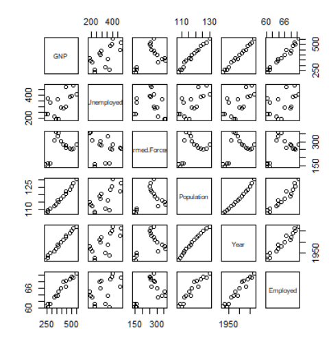
> plot(longley[, 2:7])
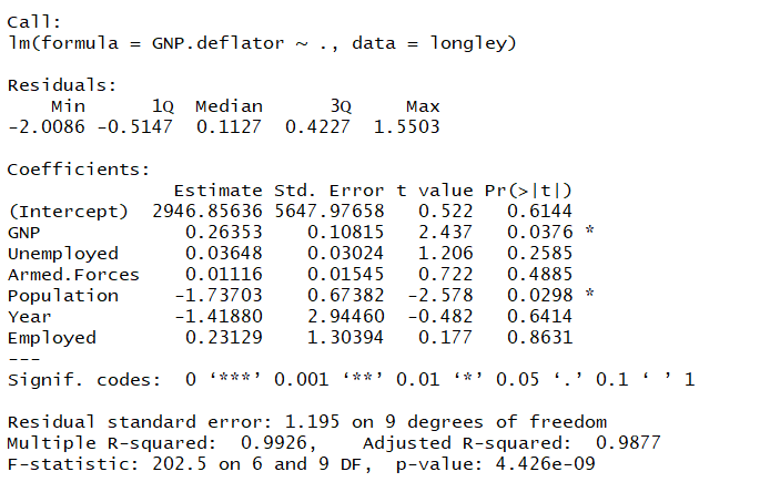

Very large VIF values are indicators of multicollinearity, here is the figure proof:
Actually from the VIF values we could still not get the straightforward access to the structure of the coexisting replations. And that is one big restriction of VIF. The independence among predictors are vital for a qualified regression model, the presence of strong multicollinearity can complicate our inferences. Here I just provide a simple method to evalueate the impact of multicollinearity, the VIF. There are still many other diagnostics available for the purpose of assessment, eigenvalue, for example. And I believe the best choice is to use multiple diagnostics that can be computed with the typical regression results in hand. I hope this file can help you.